4 - Street Networks & Web Scraping

Part 1: Visualizing crash data in Philadelphia

In this section, you will use osmnx to analyze the crash incidence in Center City.

Part 2: Scraping Craigslist

In this section, you will use Selenium and BeautifulSoup to scrape data for hundreds of apartments from Philadelphia’s Craigslist portal.

Code

import pandas as pd
import geopandas as gpd
import altair as alt
import numpy as np
from matplotlib import pyplot as plt
np.seterr(invalid="ignore");
from shapely import geometry

Part 1: Visualizing crash data in Philadelphia

1.1 Load the geometry for the region being analyzed

We’ll analyze crashes in the “Central” planning district in Philadelphia, a rough approximation for Center City. Planning districts can be loaded from Open Data Philly. Read the data into a GeoDataFrame using the following link:

http://data.phl.opendata.arcgis.com/datasets/0960ea0f38f44146bb562f2b212075aa_0.geojson

Select the “Central” district and extract the geometry polygon for only this district. After this part, you should have a polygon variable of type shapely.geometry.polygon.Polygon.

Code

url = "http://data.phl.opendata.arcgis.com/datasets/0960ea0f38f44146bb562f2b212075aa_0.geojson"
philly_districts = gpd.read_file(url).to_crs('EPSG:4326')
central = philly_districts.loc[philly_districts['DIST_NAME'] == 'Central']

polygon = central['geometry'].iloc[0]
print(type(polygon))

<class 'shapely.geometry.polygon.Polygon'>

1.2 Get the street network graph

Use OSMnx to create a network graph (of type ‘drive’) from your polygon boundary in 1.1.

Code

import osmnx as ox
graph = ox.graph_from_polygon(polygon, network_type='drive')
philly_graph = ox.project_graph(graph)
ox.plot_graph(philly_graph)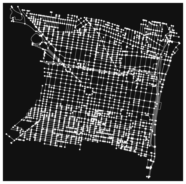

(<Figure size 800x800 with 1 Axes>, <Axes: >)

1.3 Convert your network graph edges to a GeoDataFrame

Use OSMnx to create a GeoDataFrame of the network edges in the graph object from part 1.2. The GeoDataFrame should contain the edges but not the nodes from the network.

Code

edges = ox.graph_to_gdfs(philly_graph, edges=True, nodes=False).to_crs('EPSG:4326')
edges.head()

			osmid	oneway	name	highway	reversed	length	geometry	maxspeed	lanes	tunnel	bridge	ref	width	service	access	junction
u	v	key
109727439	109911666	0	132508434	True	Bainbridge Street	residential	False	44.137	LINESTRING (-75.17104 39.94345, -75.17053 39.9...	NaN	NaN	NaN	NaN	NaN	NaN	NaN	NaN	NaN
109911666	109911655	0	132508434	True	Bainbridge Street	residential	False	45.459	LINESTRING (-75.17053 39.94339, -75.17001 39.9...	NaN	NaN	NaN	NaN	NaN	NaN	NaN	NaN	NaN
	110024009	0	12139665	True	South 17th Street	tertiary	False	109.692	LINESTRING (-75.17053 39.94339, -75.17060 39.9...	NaN	NaN	NaN	NaN	NaN	NaN	NaN	NaN	NaN
109727448	109727439	0	12109011	True	South Colorado Street	residential	False	109.484	LINESTRING (-75.17125 39.94248, -75.17120 39.9...	NaN	NaN	NaN	NaN	NaN	NaN	NaN	NaN	NaN
	110034229	0	12159387	True	Fitzwater Street	residential	False	91.353	LINESTRING (-75.17125 39.94248, -75.17137 39.9...	NaN	NaN	NaN	NaN	NaN	NaN	NaN	NaN	NaN

Code

edges.explore()

Make this Notebook Trusted to load map: File -> Trust Notebook

1.4 Load PennDOT crash data

Data for crashes (of all types) for 2020, 2021, and 2022 in Philadelphia County is available at the following path:

./data/CRASH_PHILADELPHIA_XXXX.csv

You should see three separate files in the data/ folder. Use pandas to read each of the CSV files, and combine them into a single dataframe using pd.concat().

The data was downloaded for Philadelphia County from here.

Code

crash_2020 = pd.read_csv("./data/CRASH_PHILADELPHIA_2020.csv")
crash_2021 = pd.read_csv("./data/CRASH_PHILADELPHIA_2021.csv")
crash_2022 = pd.read_csv("./data/CRASH_PHILADELPHIA_2022.csv")

Code

philly_crash = pd.concat([crash_2020, crash_2021, crash_2020])
philly_crash

	CRN	ARRIVAL_TM	AUTOMOBILE_COUNT	BELTED_DEATH_COUNT	BELTED_SUSP_SERIOUS_INJ_COUNT	BICYCLE_COUNT	BICYCLE_DEATH_COUNT	BICYCLE_SUSP_SERIOUS_INJ_COUNT	BUS_COUNT	CHLDPAS_DEATH_COUNT	...	WORK_ZONE_TYPE	WORKERS_PRES	WZ_CLOSE_DETOUR	WZ_FLAGGER	WZ_LAW_OFFCR_IND	WZ_LN_CLOSURE	WZ_MOVING	WZ_OTHER	WZ_SHLDER_MDN	WZ_WORKERS_INJ_KILLED
0	2020036588	1349.0	1	0	0	0	0	0	0	0	...	NaN	NaN	NaN	NaN	NaN	NaN	NaN	NaN	NaN	NaN
1	2020036617	1842.0	1	0	0	0	0	0	0	0	...	NaN	NaN	NaN	NaN	NaN	NaN	NaN	NaN	NaN	NaN
2	2020035717	2000.0	1	0	0	0	0	0	0	0	...	NaN	NaN	NaN	NaN	NaN	NaN	NaN	NaN	NaN	NaN
3	2020034378	1139.0	2	0	0	0	0	0	0	0	...	NaN	NaN	NaN	NaN	NaN	NaN	NaN	NaN	NaN	NaN
4	2020025511	345.0	1	0	0	0	0	0	0	0	...	NaN	NaN	NaN	NaN	NaN	NaN	NaN	NaN	NaN	NaN
...	...	...	...	...	...	...	...	...	...	...	...	...	...	...	...	...	...	...	...	...	...
10160	2020107585	2159.0	1	0	0	0	0	0	0	0	...	NaN	NaN	NaN	NaN	NaN	NaN	NaN	NaN	NaN	NaN
10161	2020109081	1945.0	2	0	0	0	0	0	0	0	...	NaN	NaN	NaN	NaN	NaN	NaN	NaN	NaN	NaN	NaN
10162	2020108478	537.0	1	0	0	0	0	0	0	0	...	NaN	NaN	NaN	NaN	NaN	NaN	NaN	NaN	NaN	NaN
10163	2020108480	2036.0	2	0	0	0	0	0	0	0	...	NaN	NaN	NaN	NaN	NaN	NaN	NaN	NaN	NaN	NaN
10164	2020110361	1454.0	0	0	0	0	0	0	0	0	...	NaN	NaN	NaN	NaN	NaN	NaN	NaN	NaN	NaN	NaN

30877 rows × 100 columns

1.5 Convert the crash data to a GeoDataFrame

You will need to use the DEC_LAT and DEC_LONG columns for latitude and longitude.

The full data dictionary for the data is available here

Code

crash_geo = gpd.GeoDataFrame(philly_crash, geometry=gpd.points_from_xy(philly_crash.DEC_LONG, philly_crash.DEC_LAT), crs="EPSG:4326")

1.6 Trim the crash data to Center City

1. Get the boundary of the edges data frame (from part 1.3). Accessing the .geometry.unary_union.convex_hull property will give you a nice outer boundary region.
2. Trim the crashes using the within() function of the crash GeoDataFrame to find which crashes are within the boundary.

There should be about 3,750 crashes within the Central district.

Code

boundary = edges.geometry.unary_union.convex_hull

central_crash = crash_geo[crash_geo.within(boundary)]
central_crash

	CRN	ARRIVAL_TM	AUTOMOBILE_COUNT	BELTED_DEATH_COUNT	BELTED_SUSP_SERIOUS_INJ_COUNT	BICYCLE_COUNT	BICYCLE_DEATH_COUNT	BICYCLE_SUSP_SERIOUS_INJ_COUNT	BUS_COUNT	CHLDPAS_DEATH_COUNT	...	WORKERS_PRES	WZ_CLOSE_DETOUR	WZ_FLAGGER	WZ_LAW_OFFCR_IND	WZ_LN_CLOSURE	WZ_MOVING	WZ_OTHER	WZ_SHLDER_MDN	WZ_WORKERS_INJ_KILLED	geometry
0	2020036588	1349.0	1	0	0	0	0	0	0	0	...	NaN	NaN	NaN	NaN	NaN	NaN	NaN	NaN	NaN	POINT (-75.17940 39.96010)
7	2020035021	1255.0	1	0	0	0	0	0	1	0	...	NaN	NaN	NaN	NaN	NaN	NaN	NaN	NaN	NaN	POINT (-75.16310 39.97000)
11	2020021944	805.0	2	0	0	0	0	0	0	0	...	NaN	NaN	NaN	NaN	NaN	NaN	NaN	NaN	NaN	POINT (-75.18780 39.95230)
12	2020024963	1024.0	1	0	0	0	0	0	0	0	...	NaN	NaN	NaN	NaN	NaN	NaN	NaN	NaN	NaN	POINT (-75.14840 39.95580)
18	2020000481	1737.0	1	0	0	0	0	0	1	0	...	NaN	NaN	NaN	NaN	NaN	NaN	NaN	NaN	NaN	POINT (-75.15470 39.95340)
...	...	...	...	...	...	...	...	...	...	...	...	...	...	...	...	...	...	...	...	...	...
10132	2020105944	1841.0	0	0	0	0	0	0	0	0	...	NaN	NaN	NaN	NaN	NaN	NaN	NaN	NaN	NaN	POINT (-75.14090 39.95380)
10133	2020112963	2052.0	2	0	0	0	0	0	0	0	...	NaN	NaN	NaN	NaN	NaN	NaN	NaN	NaN	NaN	POINT (-75.17520 39.95310)
10148	2020111219	1324.0	0	0	0	0	0	0	0	0	...	NaN	NaN	NaN	NaN	NaN	NaN	NaN	NaN	NaN	POINT (-75.16110 39.96370)
10150	2020110378	2025.0	6	0	0	0	0	0	0	0	...	NaN	NaN	NaN	NaN	NaN	NaN	NaN	NaN	NaN	POINT (-75.17770 39.94430)
10161	2020109081	1945.0	2	0	0	0	0	0	0	0	...	NaN	NaN	NaN	NaN	NaN	NaN	NaN	NaN	NaN	POINT (-75.18580 39.94150)

3926 rows × 101 columns

1.7 Re-project our data into an approriate CRS

We’ll need to find the nearest edge (street) in our graph for each crash. To do this, osmnx will calculate the distance from each crash to the graph edges. For this calculation to be accurate, we need to convert from latitude/longitude

We’ll convert the local state plane CRS for Philadelphia, EPSG=2272

Two steps:

1. Project the graph object (G) using the ox.project_graph. Run ox.project_graph? to see the documentation for how to convert to a specific CRS.
2. Project the crash data using the .to_crs() function.

Code

philly_G = ox.project_graph(philly_graph, to_crs='EPSG:2272')

Code

central_crash = central_crash.to_crs('EPSG:2272')

1.8 Find the nearest edge for each crash

See: ox.distance.nearest_edges(). It takes three arguments:

• the network graph
• the longitude of your crash data (the x attribute of the geometry column)
• the latitude of your crash data (the y attribute of the geometry column)

You will get a numpy array with 3 columns that represent (u, v, key) where each u and v are the node IDs that the edge links together. We will ignore the key value for our analysis.

Code

nearest_crash = ox.distance.nearest_edges(philly_G, central_crash['geometry'].x, central_crash['geometry'].y)

1.9 Calculate the total number of crashes per street

1. Make a DataFrame from your data from part 1.7 with three columns, u, v, and key (we will only use the u and v columns)
2. Group by u and v and calculate the size
3. Reset the index and name your size() column as crash_count

After this step you should have a DataFrame with three columns: u, v, and crash_count.

Code

nearest_Crash = pd.DataFrame(nearest_crash, columns=['u', 'v', 'key'])

Code

crash_counts = nearest_Crash.groupby(['u', 'v']).count().reset_index()
crash_counts = crash_counts.rename(columns={'key': 'crash_count'})
crash_counts

	u	v	crash_count
0	109729474	3425014859	2
1	109729486	110342146	4
2	109729699	109811674	10
3	109729709	109729731	3
4	109729731	109729739	6
...	...	...	...
729	10270051289	5519334546	1
730	10660521823	10660521817	2
731	10674041689	10674041689	14
732	11144117753	109729699	4
733	11162290432	110329835	1

734 rows × 3 columns

1.10 Merge your edges GeoDataFrame and crash count DataFrame

You can use pandas to merge them on the u and v columns. This will associate the total crash count with each edge in the street network.

Tips: - Use a left merge where the first argument of the merge is the edges GeoDataFrame. This ensures no edges are removed during the merge. - Use the fillna(0) function to fill in missing crash count values with zero.

Code

merged = pd.merge(edges, crash_counts, on=['u','v'], how='left').fillna(0)
merged.head()

	u	v	osmid	oneway	name	highway	reversed	length	geometry	maxspeed	lanes	tunnel	bridge	ref	width	service	access	junction	crash_count
0	109727439	109911666	132508434	True	Bainbridge Street	residential	False	44.137	LINESTRING (-75.17104 39.94345, -75.17053 39.9...	0	0	0	0	0	0	0	0	0	0.0
1	109911666	109911655	132508434	True	Bainbridge Street	residential	False	45.459	LINESTRING (-75.17053 39.94339, -75.17001 39.9...	0	0	0	0	0	0	0	0	0	0.0
2	109911666	110024009	12139665	True	South 17th Street	tertiary	False	109.692	LINESTRING (-75.17053 39.94339, -75.17060 39.9...	0	0	0	0	0	0	0	0	0	0.0
3	109727448	109727439	12109011	True	South Colorado Street	residential	False	109.484	LINESTRING (-75.17125 39.94248, -75.17120 39.9...	0	0	0	0	0	0	0	0	0	0.0
4	109727448	110034229	12159387	True	Fitzwater Street	residential	False	91.353	LINESTRING (-75.17125 39.94248, -75.17137 39.9...	0	0	0	0	0	0	0	0	0	0.0

1.11 Calculate a “Crash Index”

Let’s calculate a “crash index” that provides a normalized measure of the crash frequency per street. To do this, we’ll need to:

1. Calculate the total crash count divided by the street length, using the length column
2. Perform a log transformation of the crash/length variable — use numpy’s log10() function
3. Normalize the index from 0 to 1 (see the lecture notes for an example of this transformation)

Note: since the crash index involves a log transformation, you should only calculate the index for streets where the crash count is greater than zero.

After this step, you should have a new column in the data frame from 1.9 that includes a column called part 1.9.

Code

merge_dropna = merged[merged['crash_count'] != 0]

Code

calculation = np.log10(merge_dropna['crash_count']/merge_dropna['length'])
#(np.log10(merged['crash_count']/merged['length']) - np.log10(merged['crash_count']/merged['length']).min())/ (np.log10(merged['crash_count']/merged['length']).max() - np.log10(merged['crash_count']/merged['length']).min())
merge_dropna['crash index'] = (calculation - calculation.min())/(calculation.max() - calculation.min())
merge_dropna.head(5)

/Users/annzhang/mambaforge/envs/musa-550-fall-2023/lib/python3.10/site-packages/geopandas/geodataframe.py:1538: SettingWithCopyWarning: 
A value is trying to be set on a copy of a slice from a DataFrame.
Try using .loc[row_indexer,col_indexer] = value instead

See the caveats in the documentation: https://pandas.pydata.org/pandas-docs/stable/user_guide/indexing.html#returning-a-view-versus-a-copy
  super().__setitem__(key, value)

	u	v	osmid	oneway	name	highway	reversed	length	geometry	maxspeed	lanes	tunnel	bridge	ref	width	service	access	junction	crash_count	crash index
9	110024052	110024066	12139665	True	South 17th Street	tertiary	False	135.106	LINESTRING (-75.17134 39.93966, -75.17152 39.9...	0	0	0	0	0	0	0	0	0	9.0	0.431858
30	109729474	3425014859	62154356	True	Arch Street	secondary	False	126.087	LINESTRING (-75.14847 39.95259, -75.14859 39.9...	25 mph	2	0	0	0	0	0	0	0	2.0	0.258123
31	109729486	110342146	[12169305, 1052694387]	True	North Independence Mall East	secondary	False	123.116	LINESTRING (-75.14832 39.95333, -75.14813 39.9...	0	[3, 2]	0	0	0	0	0	0	0	4.0	0.344930
33	3425014859	5372059859	[12197696, 1003976882, 424804083]	True	North Independence Mall West	secondary	False	229.386	LINESTRING (-75.14993 39.95277, -75.14995 39.9...	0	3	0	0	0	0	0	0	0	2.0	0.185670
35	110342146	315655546	[424807270, 12109183]	True	0	motorway_link	False	153.933	LINESTRING (-75.14809 39.95442, -75.14808 39.9...	0	1	0	0	0	0	0	0	0	3.0	0.283054

1.12 Plot a histogram of the crash index values

Use matplotlib’s hist() function to plot the crash index values from the previous step.

You should see that the index values are Gaussian-distributed, providing justification for why we log-transformed!

Code

plt.hist(merge_dropna['crash index'], color='pink', bins=20)

plt.xlabel('Crash Index')
plt.ylabel('Frequency')
plt.title('Crash Index Values Histogram')
plt.show()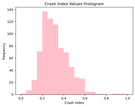

1.13 Plot an interactive map of the street networks, colored by the crash index

You can use GeoPandas to make an interactive Folium map, coloring the streets by the crash index column.

Tip: if you use the viridis color map, try using a “dark” tile set for better constrast of the colors.

Code

crash_index = merge_dropna[['u', 'v', 'crash index']]
merged_index = pd.merge(merged, crash_index, on=['u','v'], how='left').fillna(0)

Code

merged_index.explore(
    column="crash index",
    cmap="YlGnBu",
    tiles="cartodbpositron",)

Make this Notebook Trusted to load map: File -> Trust Notebook

Part 2: Scraping Craigslist

In this part, we’ll be extracting information on apartments from Craigslist search results. You’ll be using Selenium and BeautifulSoup to extract the relevant information from the HTML text.

For reference on CSS selectors, please see the notes from Week 6.

Primer: the Craigslist website URL

We’ll start with the Philadelphia region. First we need to figure out how to submit a query to Craigslist. As with many websites, one way you can do this is simply by constructing the proper URL and sending it to Craigslist.

https://philadelphia.craigslist.org/search/apa?min_price=1&min_bedrooms=1&minSqft=1#search=1_gallery0~0

There are three components to this URL.

1. The base URL: http://philadelphia.craigslist.org/search/apa

2. The user’s search parameters: ?min_price=1&min_bedrooms=1&minSqft=1

We will send nonzero defaults for some parameters (bedrooms, size, price) in order to exclude results that have empty values for these parameters.

3. The URL hash: #search=1~gallery~0~0

As we will see later, this part will be important because it contains the search page result number.

The Craigslist website requires Javascript, so we’ll need to use Selenium to load the page, and then use BeautifulSoup to extract the information we want.

2.1 Initialize a selenium driver and open Craigslist

As discussed in lecture, you can use Chrome, Firefox, or Edge as your selenium driver. In this part, you should do two things:

1. Initialize the selenium driver
2. Use the driver.get() function to open the following URL:

https://philadelphia.craigslist.org/search/apa?min_price=1&min_bedrooms=1&minSqft=1#search=1_gallery0~0

This will give you the search results for 1-bedroom apartments in Philadelphia.

Code

from selenium import webdriver
from bs4 import BeautifulSoup
import requests

Code

driver = webdriver.Chrome()
url = "https://philadelphia.craigslist.org/search/apa?min_price=1&min_bedrooms=1&minSqft=1#search=1~gallery~0~0"
driver.get(url)

2.2 Initialize your “soup”

Once selenium has the page open, we can get the page source from the driver and use BeautifulSoup to parse it. In this part, initialize a BeautifulSoup object with the driver’s page source

Code

soup = BeautifulSoup(driver.page_source, "html.parser")

2.3 Parsing the HTML

Now that we have our “soup” object, we can use BeautifulSoup to extract out the elements we need:

• Use the Web Inspector to identify the HTML element that holds the information on each apartment listing.
• Use BeautifulSoup to extract these elements from the HTML.

At the end of this part, you should have a list of 120 elements, where each element is the listing for a specific apartment on the search page.

Code

selector = ".cl-search-result.cl-search-view-mode-gallery"

tables = soup.select(selector)

Code

len(tables)

120

2.4 Find the relevant pieces of information

We will now focus on the first element in the list of 120 apartments. Use the prettify() function to print out the HTML for this first element.

From this HTML, identify the HTML elements that hold:

• The apartment price
• The number of bedrooms
• The square footage
• The apartment title

For the first apartment, print out each of these pieces of information, using BeautifulSoup to select the proper elements.

Code

print(tables[1].prettify())

<li class="cl-search-result cl-search-view-mode-gallery" data-pid="7681605868" title="Apartment by the arts!">
 <div class="gallery-card">
  <div class="cl-gallery">
   <div class="gallery-inner">
    <a class="main" href="https://philadelphia.craigslist.org/apa/d/philadelphia-apartment-by-the-arts/7681605868.html">
     <div class="swipe" style="visibility: visible;">
      <div class="swipe-wrap" style="width: 4032px;">
       <div data-index="0" style="width: 336px; left: 0px; transition-duration: 0ms; transform: translateX(0px);">
        <span class="loading icom-">
        </span>
        <img alt="Apartment by the arts! 1" src="https://images.craigslist.org/00j0j_bWLeLp3Yzpi_0x20m2_300x300.jpg"/>
       </div>
       <div data-index="1" style="width: 336px; left: -336px; transition-duration: 0ms; transform: translateX(336px);">
       </div>
       <div data-index="2" style="width: 336px; left: -672px; transition-duration: 0ms; transform: translateX(336px);">
       </div>
       <div data-index="3" style="width: 336px; left: -1008px; transition-duration: 0ms; transform: translateX(336px);">
       </div>
       <div data-index="4" style="width: 336px; left: -1344px; transition-duration: 0ms; transform: translateX(336px);">
       </div>
       <div data-index="5" style="width: 336px; left: -1680px; transition-duration: 0ms; transform: translateX(-336px);">
       </div>
      </div>
     </div>
     <div class="slider-back-arrow icom-">
     </div>
     <div class="slider-forward-arrow icom-">
     </div>
    </a>
   </div>
   <div class="dots">
    <span class="dot selected">
     •
    </span>
    <span class="dot">
     •
    </span>
    <span class="dot">
     •
    </span>
    <span class="dot">
     •
    </span>
    <span class="dot">
     •
    </span>
    <span class="dot">
     •
    </span>
   </div>
  </div>
  <a class="cl-app-anchor text-only posting-title" href="https://philadelphia.craigslist.org/apa/d/philadelphia-apartment-by-the-arts/7681605868.html" tabindex="0">
   <span class="label">
    Apartment by the arts!
   </span>
  </a>
  <div class="meta">
   14 mins ago
   <span class="separator">
    ·
   </span>
   <span class="housing-meta">
    <span class="post-bedrooms">
     2br
    </span>
    <span class="post-sqft">
     1390ft
     <span class="exponent">
      2
     </span>
    </span>
   </span>
   <span class="separator">
    ·
   </span>
   Philadelphia
  </div>
  <span class="priceinfo">
   $2,850
  </span>
  <button class="bd-button cl-favorite-button icon-only" tabindex="0" title="add to favorites list" type="button">
   <span class="icon icom-">
   </span>
   <span class="label">
   </span>
  </button>
  <button class="bd-button cl-banish-button icon-only" tabindex="0" title="hide posting" type="button">
   <span class="icon icom-">
   </span>
   <span class="label">
    hide
   </span>
  </button>
 </div>
</li>

Code

table = tables[1]

Code

data = []

#price
price = table.select_one(".priceinfo").text

#no. of bedrooms
bedrooms = table.select_one(".post-bedrooms").text
    
#square footage
size = table.select_one(".post-sqft").text
    
#apt name
name = table.select_one(".label").text

data.append({"Price": price, "Bedrooms": bedrooms, "Size": size, "Name": name})

data = pd.DataFrame(data)

data

	Price	Bedrooms	Size	Name
0	$2,850	2br	1390ft2	Apartment by the arts!

2.5 Functions to format the results

In this section, you’ll create functions that take in the raw string elements for price, size, and number of bedrooms and returns them formatted as numbers.

I’ve started the functions to format the values. You should finish theses functions in this section.

Hints - You can use string formatting functions like string.replace() and string.strip() - The int() and float() functions can convert strings to numbers

Code

def format_bedrooms(bedrooms_string):
    
    bedrooms = int(bedrooms_string.replace("br", ""))
    
    return bedrooms

Code

def format_size(size_string):
    
    size = int(size_string.replace("ft", ""))
    
    return size 

Code

def format_price(price_string):
    
    price = int(price_string.replace("$", "").replace("," , ""))
    
    return price

2.6 Putting it all together

In this part, you’ll complete the code block below using results from previous parts. The code will loop over 5 pages of search results and scrape data for 600 apartments.

We can get a specific page by changing the search=PAGE part of the URL hash. For example, to get page 2 instead of page 1, we will navigate to:

https://philadelphia.craigslist.org/search/apa?min_price=1&min_bedrooms=1&minSqft=1#search=2_gallery0~0

In the code below, the outer for loop will loop over 5 pages of search results. The inner for loop will loop over the 120 apartments listed on each search page.

Fill in the missing pieces of the inner loop using the code from the previous section. We will be able to extract out the relevant pieces of info for each apartment.

After filling in the missing pieces and executing the code cell, you should have a Data Frame called results that holds the data for 600 apartment listings.

Notes

Be careful if you try to scrape more listings. Craigslist will temporarily ban your IP address (for a very short time) if you scrape too much at once. I’ve added a sleep() function to the for loop to wait 30 seconds between scraping requests.

If the for loop gets stuck at the “Processing page X…” step for more than a minute or so, your IP address is probably banned temporarily, and you’ll have to wait a few minutes before trying again.

Code

from time import sleep

Code

results = []

# search in batches of 120 for 5 pages
# NOTE: you will get temporarily banned if running more than ~5 pages or so
# the API limits are more leninient during off-peak times, and you can try
# experimenting with more pages
max_pages = 5

# The base URL we will be using
base_url = "https://philadelphia.craigslist.org/search/apa?min_price=1&min_bedrooms=1&minSqft=1"

# loop over each page of search results
for page_num in range(1, max_pages + 1):
    print(f"Processing page {page_num}...")

    # Update the URL hash for this page number and make the combined URL
    url_hash = f"#search={page_num}~gallery~0~0"
    url = base_url + url_hash

    # Go to the driver and wait for 5 seconds
    driver.get(url)
    sleep(5)

    # YOUR CODE: get the list of all apartments
    # This is the same code from Part 1.2 and 1.3
    # It should be a list of 120 apartments
    soup = soup
    apts = tables
    print("Number of apartments = ", len(apts))

    # loop over each apartment in the list
    page_results = []
    for apt in apts:

        # YOUR CODE: the bedrooms string
        bedrooms = apt.select_one(".post-bedrooms").text

        # YOUR CODE: the size string
        size = apt.select_one(".post-sqft").text

        # YOUR : the title string
        title = apt.select_one(".label").text

        # YOUR CODE: the price string
        price = apt.select_one(".priceinfo").text


        # Format using functions from Part 1.5
        bedrooms = format_bedrooms(bedrooms)
        size = format_size(size)
        price = format_price(price)

        # Save the result
        page_results.append([price, size, bedrooms, title])

    # Create a dataframe and save
    col_names = ["price", "size", "bedrooms", "title"]
    df = pd.DataFrame(page_results, columns=col_names)
    results.append(df)

    print("sleeping for 10 seconds between calls")
    sleep(10)

# Finally, concatenate all the results
results = pd.concat(results, axis=0).reset_index(drop=True)

Processing page 1...
Number of apartments =  120
sleeping for 10 seconds between calls
Processing page 2...
Number of apartments =  120
sleeping for 10 seconds between calls
Processing page 3...
Number of apartments =  120
sleeping for 10 seconds between calls
Processing page 4...
Number of apartments =  120
sleeping for 10 seconds between calls
Processing page 5...
Number of apartments =  120
sleeping for 10 seconds between calls

Code

results

	price	size	bedrooms	title	pricepersq
0	2474	13942	3	3bd 2ba, Serene Wooded View, West Chester PA	0.177449
1	2850	13902	2	Apartment by the arts!	0.205006
2	1800	7592	1	A Cozy Living Space In Rittenhouse Square.	0.237092
3	1750	5002	1	Pets welcome in this Beautifully renovated apa...	0.349860
4	1950	8502	2	Enjoy a fantastic living space with tons of na...	0.229358
...	...	...	...	...	...
595	2075	12712	2	Resort-Style Swimming Pool, Extra Storage, 2/BD	0.163232
596	1876	5072	1	On-demand car wash/detailing, Handyman and mai...	0.369874
597	1680	5092	1	Penthouse Hideaway, LVT Flooring, Bike Storage	0.329929
598	2199	6922	1	Fire Pit, On-site Management/Maintenance, Flex...	0.317683
599	1544	5182	1	1 BD, Bike Storage, Washer/Dryer	0.297954

600 rows × 5 columns

2.7 Plotting the distribution of prices

Use matplotlib’s hist() function to make two histograms for:

• Apartment prices
• Apartment prices per square foot (price / size)

Make sure to add labels to the respective axes and a title describing the plot.

Code

plt.title('Apartment Price Distributions')
plt.hist(results['price'], color='pink', edgecolor='grey')
plt.xlabel('Price ($)')
plt.ylabel('Counts')
plt.show()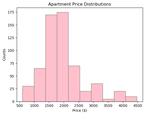

Code

results['pricepersq'] = results['price'] / results['size']

plt.title('Apartment Price Per Square foot')
plt.hist(results['pricepersq'], color='lightgrey', edgecolor='grey')
plt.xlabel('Price per sqft($)')
plt.ylabel('Counts')
plt.show()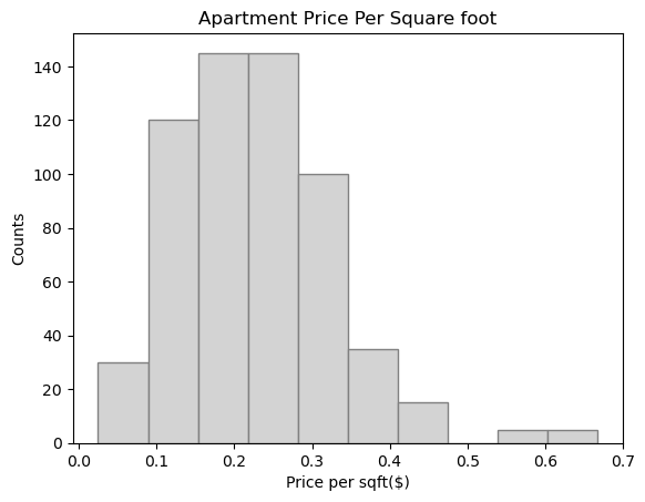

Side note: rental prices per sq. ft. from Craigslist

The histogram of price per sq ft should be centered around ~1.5. Here is a plot of how Philadelphia’s rents compare to the other most populous cities:

Source

2.8 Comparing prices for different sizes

Use altair to explore the relationship between price, size, and number of bedrooms. Make an interactive scatter plot of price (x-axis) vs. size (y-axis), with the points colored by the number of bedrooms.

Make sure the plot is interactive (zoom-able and pan-able) and add a tooltip with all of the columns in our scraped data frame.

With this sort of plot, you can quickly see the outlier apartments in terms of size and price.

Code

chart = alt.Chart(results)
chart = chart.mark_circle(size=40)
chart = chart.encode(
    x = "price:Q",
    y = "size:Q",
    color = "bedrooms:N",
    tooltip = ["title", "price", "size", "bedrooms"],
)

chart.interactive()